Lorem ipsum dolor sit amet, consectetur adipisicing elit. Odit molestiae mollitia laudantium assumenda nam eaque, excepturi, soluta, perspiciatis cupiditate sapiente, adipisci quaerat odio voluptates consectetur nulla eveniet iure vitae quibusdam? Excepturi aliquam in iure, repellat, fugiat illum voluptate repellendus blanditiis veritatis ducimus ad ipsa quisquam, commodi vel necessitatibus, harum quos a dignissimos.
Close Save changesHelp F1 or ? Previous Page ← + CTRL (Windows) ← + ⌘ (Mac) Next Page → + CTRL (Windows) → + ⌘ (Mac) Search Site CTRL + SHIFT + F (Windows) ⌘ + ⇧ + F (Mac) Close Message ESC
The P-value approach involves determining "likely" or "unlikely" by determining the probability — assuming the null hypothesis was true — of observing a more extreme test statistic in the direction of the alternative hypothesis than the one observed. If the P-value is small, say less than (or equal to) \(\alpha\), then it is "unlikely." And, if the P-value is large, say more than \(\alpha\), then it is "likely."
If the P-value is less than (or equal to) \(\alpha\), then the null hypothesis is rejected in favor of the alternative hypothesis. And, if the P-value is greater than \(\alpha\), then the null hypothesis is not rejected.
Specifically, the four steps involved in using the P-value approach to conducting any hypothesis test are:
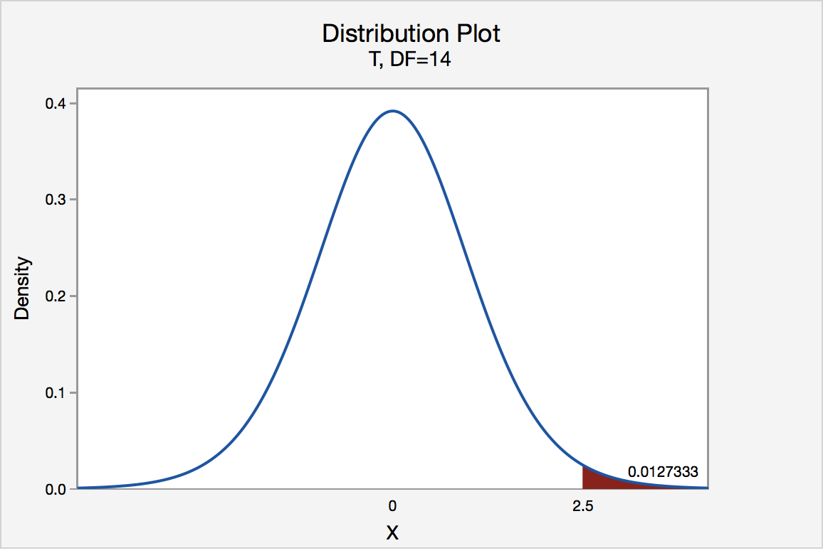
In our example concerning the mean grade point average, suppose that our random sample of n = 15 students majoring in mathematics yields a test statistic t* equaling 2.5. Since n = 15, our test statistic t* has n - 1 = 14 degrees of freedom. Also, suppose we set our significance level α at 0.05 so that we have only a 5% chance of making a Type I error.
The P-value for conducting the right-tailed test H 0 : μ = 3 versus H A : μ > 3 is the probability that we would observe a test statistic greater than t* = 2.5 if the population mean \(\mu\) really were 3. Recall that probability equals the area under the probability curve. The P-value is therefore the area under a t n - 1 = t 14 curve and to the right of the test statistic t* = 2.5. It can be shown using statistical software that the P-value is 0.0127. The graph depicts this visually.
The P-value, 0.0127, tells us it is "unlikely" that we would observe such an extreme test statistic t* in the direction of H A if the null hypothesis were true. Therefore, our initial assumption that the null hypothesis is true must be incorrect. That is, since the P-value, 0.0127, is less than \(\alpha\) = 0.05, we reject the null hypothesis H 0 : μ = 3 in favor of the alternative hypothesis H A : μ > 3.
Note that we would not reject H 0 : μ = 3 in favor of H A : μ > 3 if we lowered our willingness to make a Type I error to \(\alpha\) = 0.01 instead, as the P-value, 0.0127, is then greater than \(\alpha\) = 0.01.
In our example concerning the mean grade point average, suppose that our random sample of n = 15 students majoring in mathematics yields a test statistic t* instead of equaling -2.5. The P-value for conducting the left-tailed test H 0 : μ = 3 versus H A : μ < 3 is the probability that we would observe a test statistic less than t* = -2.5 if the population mean μ really were 3. The P-value is therefore the area under a t n - 1 = t 14 curve and to the left of the test statistic t* = -2.5. It can be shown using statistical software that the P-value is 0.0127. The graph depicts this visually.
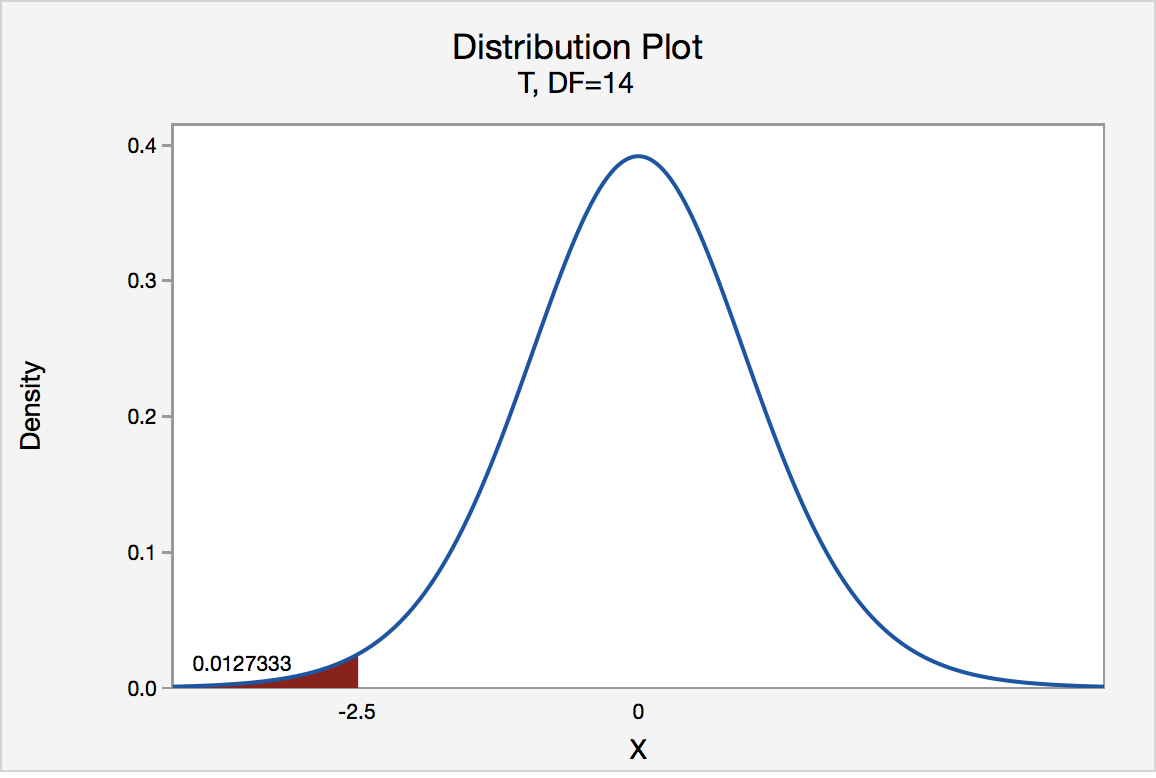
The P-value, 0.0127, tells us it is "unlikely" that we would observe such an extreme test statistic t* in the direction of H A if the null hypothesis were true. Therefore, our initial assumption that the null hypothesis is true must be incorrect. That is, since the P-value, 0.0127, is less than α = 0.05, we reject the null hypothesis H 0 : μ = 3 in favor of the alternative hypothesis H A : μ < 3.
In our example concerning the mean grade point average, suppose again that our random sample of n = 15 students majoring in mathematics yields a test statistic t* instead of equaling -2.5. The P-value for conducting the two-tailed test H 0 : μ = 3 versus H A : μ ≠ 3 is the probability that we would observe a test statistic less than -2.5 or greater than 2.5 if the population mean μ really was 3. That is, the two-tailed test requires taking into account the possibility that the test statistic could fall into either tail (hence the name "two-tailed" test). The P-value is, therefore, the area under a t n - 1 = t 14 curve to the left of -2.5 and to the right of 2.5. It can be shown using statistical software that the P-value is 0.0127 + 0.0127, or 0.0254. The graph depicts this visually.
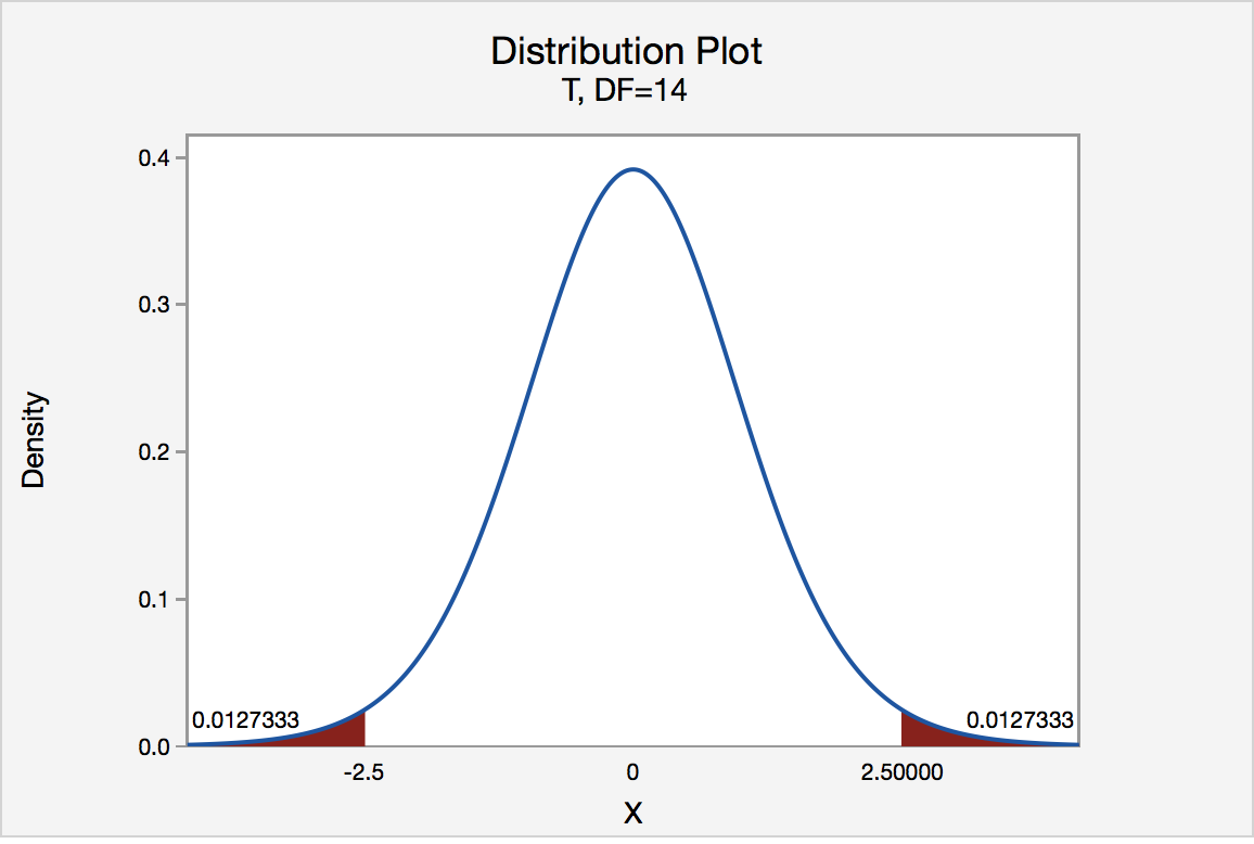
Note that the P-value for a two-tailed test is always two times the P-value for either of the one-tailed tests. The P-value, 0.0254, tells us it is "unlikely" that we would observe such an extreme test statistic t* in the direction of H A if the null hypothesis were true. Therefore, our initial assumption that the null hypothesis is true must be incorrect. That is, since the P-value, 0.0254, is less than α = 0.05, we reject the null hypothesis H 0 : μ = 3 in favor of the alternative hypothesis H A : μ ≠ 3.
Note that we would not reject H 0 : μ = 3 in favor of H A : μ ≠ 3 if we lowered our willingness to make a Type I error to α = 0.01 instead, as the P-value, 0.0254, is then greater than \(\alpha\) = 0.01.
Now that we have reviewed the critical value and P-value approach procedures for each of the three possible hypotheses, let's look at three new examples — one of a right-tailed test, one of a left-tailed test, and one of a two-tailed test.
The good news is that, whenever possible, we will take advantage of the test statistics and P-values reported in statistical software, such as Minitab, to conduct our hypothesis tests in this course.